Parallel Training Optimization
We use hybrid optimization to train the 🐸STT model across multiple GPUs on a single host. Parallel optimization can take on various forms. For example one can use asynchronous updates of the model, synchronous updates of the model, or some combination of the two.
Asynchronous Parallel Optimization
In asynchronous parallel optimization, for example, one places the model initially in CPU memory. Then each of the \(G\) GPUs obtains a mini-batch of data along with the current model parameters. Using this mini-batch each GPU then computes the gradients for all model parameters and sends these gradients back to the CPU when the GPU is done with its mini-batch. The CPU then asynchronously updates the model parameters whenever it receives a set of gradients from a GPU.
Asynchronous parallel optimization has several advantages and several disadvantages. One large advantage is throughput. No GPU will ever be waiting idle. When a GPU is done processing a mini-batch, it can immediately obtain the next mini-batch to process. It never has to wait on other GPUs to finish their mini-batch. However, this means that the model updates will also be asynchronous which can have problems.
For example, one may have model parameters \(W\) on the CPU and send mini-batch \(n\) to GPU 1 and send mini-batch \(n+1\) to GPU 2. As processing is asynchronous, GPU 2 may finish before GPU 1 and thus update the CPU’s model parameters \(W\) with its gradients \(\Delta W_{n+1}(W)\), where the subscript \(n+1\) identifies the mini-batch and the argument \(W\) the location at which the gradient was evaluated.
This results in the new model parameters:
Next GPU 1 could finish with its mini-batch and update the parameters to
The problem with this is that \(\Delta W_{n}(W)\) is evaluated at \(W\) and not \(W + \Delta W_{n+1}(W)\). Hence, the direction of the gradient \(\Delta W_{n}(W)\) is slightly incorrect as it is evaluated at the wrong location. This can be counteracted through synchronous updates of model, but this is also problematic.
Synchronous Optimization
Synchronous optimization solves the problem we saw above. In synchronous optimization, one places the model initially in CPU memory. Then one of the G GPUs is given a mini-batch of data along with the current model parameters. Using the mini-batch the GPU computes the gradients for all model parameters and sends the gradients back to the CPU. The CPU then updates the model parameters and starts the process of sending out the next mini-batch.
As on can readily see, synchronous optimization does not have the problem we found in the last section, that of incorrect gradients. However, synchronous optimization can only make use of a single GPU at a time. So, when we have a multi-GPU setup, \(G > 1\), all but one of the GPUs will remain idle, which is unacceptable. However, there is a third alternative which is combines the advantages of asynchronous and synchronous optimization.
Hybrid Parallel Optimization
Hybrid parallel optimization combines most of the benefits of asynchronous and synchronous optimization. It allows for multiple GPUs to be used, but does not suffer from the incorrect gradient problem exhibited by asynchronous optimization.
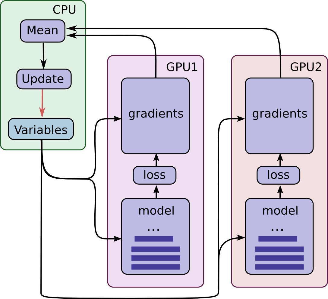
In hybrid parallel optimization one places the model initially in CPU memory. Then, as in asynchronous optimization, each of the \(G\) GPUs obtains a mini-batch of data along with the current model parameters. Using the mini-batch each of the GPUs then computes the gradients for all model parameters and sends these gradients back to the CPU. Now, in contrast to asynchronous optimization, the CPU waits until each GPU is finished with its mini-batch then takes the mean of all the gradients from the \(G\) GPUs and updates the model with this mean gradient.
Hybrid parallel optimization has several advantages and few disadvantages. As in asynchronous parallel optimization, hybrid parallel optimization allows for one to use multiple GPUs in parallel. Furthermore, unlike asynchronous parallel optimization, the incorrect gradient problem is not present here. In fact, hybrid parallel optimization performs as if one is working with a single mini-batch which is \(G\) times the size of a mini-batch handled by a single GPU. However, hybrid parallel optimization is not perfect. If one GPU is slower than all the others in completing its mini-batch, all other GPUs will have to sit idle until this straggler finishes with its mini-batch. This hurts throughput. But, if all GPUs are of the same make and model, this problem should be minimized.
So, relatively speaking, hybrid parallel optimization seems the have more advantages and fewer disadvantages as compared to both asynchronous and synchronous optimization. So, we will, for our work, use this hybrid model.
Adam Optimization
In contrast to Deep Speech: Scaling up end-to-end speech recognition, in which Nesterov’s Accelerated Gradient Descent was used, we use the Adam method for optimization, because in our experience the latter requires less fine-tuning.